R
Machine Learning
Autor/a

Joel Burbano

Fecha de publicación

27 de agosto de 2024

En este proyecto vamos a desarrollar un modelo predictivo para identificar clientes con alto riesgo de churn (abandono) en una institución bancaria, utilizando técnicas de Machine Learning

Importación de Datos

Código
# Importamos las librerias
library(data.table)
library(tidyverse)
source("D:/Joel/Blog/recursos/funciones_aux.R")
df <- fread("Churn_Modelling.csv")
head(df,5)
   RowNumber CustomerId  Surname CreditScore Geography Gender   Age Tenure
       <int>      <int>   <char>       <int>    <char> <char> <num>  <int>
1:         1   15634602 Hargrave         619    France Female    42      2
2:         2   15647311     Hill         608     Spain Female    41      1
3:         3   15619304     Onio         502    France Female    42      8
4:         4   15701354     Boni         699    France Female    39      1
5:         5   15737888 Mitchell         850     Spain Female    43      2
     Balance NumOfProducts HasCrCard IsActiveMember EstimatedSalary Exited
       <num>         <int>     <int>          <int>           <num>  <int>
1:      0.00             1         1              1       101348.88      1
2:  83807.86             1         0              1       112542.58      0
3: 159660.80             3         1              0       113931.57      1
4:      0.00             2         0              0        93826.63      0
5: 125510.82             1        NA              1        79084.10      0

breve revisión a la variable dependiente

Código
df[, .N, by = Exited]
   Exited     N
    <int> <int>
1:      1  2038
2:      0  7964

Notamos que la data esta desbalanceada con el grupo mayoritario 1 que son las personas que abandonan

  • 0 No abandona
  • 1 Abandona

Particionamos la data en conjuntos Train / Test

Código
# Base de modelamiento / validacion
set.seed(95)
marca <- sample(1:nrow(df), size = floor(0.7 * nrow(df)), replace = FALSE)
df[, ModVal := 1:nrow(df)]
df[, ModVal := ifelse(ModVal %in% marca, 0, 1)]
df[, .N, by = ModVal]
   ModVal     N
    <num> <int>
1:      1  3001
2:      0  7001
Código
df[, table(Exited, ModVal, useNA = "always")]
      ModVal
Exited    0    1 <NA>
  0    5548 2416    0
  1    1453  585    0
  <NA>    0    0    0

Análisis Exploratorio

Tipo de datos

Código
str(df)
Classes 'data.table' and 'data.frame':  10002 obs. of  15 variables:
 $ RowNumber      : int  1 2 3 4 5 6 7 8 9 10 ...
 $ CustomerId     : int  15634602 15647311 15619304 15701354 15737888 15574012 15592531 15656148 15792365 15592389 ...
 $ Surname        : chr  "Hargrave" "Hill" "Onio" "Boni" ...
 $ CreditScore    : int  619 608 502 699 850 645 822 376 501 684 ...
 $ Geography      : chr  "France" "Spain" "France" "France" ...
 $ Gender         : chr  "Female" "Female" "Female" "Female" ...
 $ Age            : num  42 41 42 39 43 44 50 29 44 NA ...
 $ Tenure         : int  2 1 8 1 2 8 7 4 4 2 ...
 $ Balance        : num  0 83808 159661 0 125511 ...
 $ NumOfProducts  : int  1 1 3 2 1 2 2 4 2 1 ...
 $ HasCrCard      : int  1 0 1 0 NA 1 1 1 0 1 ...
 $ IsActiveMember : int  1 1 0 0 1 0 1 0 NA 1 ...
 $ EstimatedSalary: num  101349 112543 113932 93827 79084 ...
 $ Exited         : int  1 0 1 0 0 1 0 1 0 0 ...
 $ ModVal         : num  1 0 0 0 0 0 1 0 0 1 ...
 - attr(*, ".internal.selfref")=<externalptr> 

creamos una lista de variables para mejor manipulación

Código
index <- c("RowNumber", "CustomerId","Surname")
var_num <- c("CreditScore", "Age", "Tenure", "Balance","EstimatedSalary")
var_cat <- setdiff(names(df),c(index,var_num,"Exited"))

Cambio de nombres de las columnas

En esta ocasión no vamos a cambiar ningun nombre

Exploración de datos

Primero visualicemos un breve resumen de las variables

Código
summary(df)
   RowNumber       CustomerId         Surname           CreditScore   
 Min.   :    1   Min.   :15565701   Length:10002       Min.   :350.0  
 1st Qu.: 2501   1st Qu.:15628525   Class :character   1st Qu.:584.0  
 Median : 5002   Median :15690732   Mode  :character   Median :652.0  
 Mean   : 5002   Mean   :15690933                      Mean   :650.6  
 3rd Qu.: 7502   3rd Qu.:15753226                      3rd Qu.:718.0  
 Max.   :10000   Max.   :15815690                      Max.   :850.0  
                                                                      
  Geography            Gender               Age            Tenure      
 Length:10002       Length:10002       Min.   :18.00   Min.   : 0.000  
 Class :character   Class :character   1st Qu.:32.00   1st Qu.: 3.000  
 Mode  :character   Mode  :character   Median :37.00   Median : 5.000  
                                       Mean   :38.92   Mean   : 5.012  
                                       3rd Qu.:44.00   3rd Qu.: 7.000  
                                       Max.   :92.00   Max.   :10.000  
                                       NA's   :1                       
    Balance       NumOfProducts    HasCrCard      IsActiveMember  
 Min.   :     0   Min.   :1.00   Min.   :0.0000   Min.   :0.0000  
 1st Qu.:     0   1st Qu.:1.00   1st Qu.:0.0000   1st Qu.:0.0000  
 Median : 97199   Median :1.00   Median :1.0000   Median :1.0000  
 Mean   : 76491   Mean   :1.53   Mean   :0.7055   Mean   :0.5149  
 3rd Qu.:127648   3rd Qu.:2.00   3rd Qu.:1.0000   3rd Qu.:1.0000  
 Max.   :250898   Max.   :4.00   Max.   :1.0000   Max.   :1.0000  
                                 NA's   :1        NA's   :1       
 EstimatedSalary         Exited           ModVal   
 Min.   :    11.58   Min.   :0.0000   Min.   :0.0  
 1st Qu.: 50983.75   1st Qu.:0.0000   1st Qu.:0.0  
 Median :100185.24   Median :0.0000   Median :0.0  
 Mean   :100083.33   Mean   :0.2038   Mean   :0.3  
 3rd Qu.:149383.65   3rd Qu.:0.0000   3rd Qu.:1.0  
 Max.   :199992.48   Max.   :1.0000   Max.   :1.0  
                                                   

Notamos que existen valores perdidos o NA’s, los mismos que serán tratados mas adelante

Evaluación de valores nulos

Código
# tratamiento NA's 
df <- df[!(is.na(HasCrCard) == TRUE),]
df <- df[!(is.na(IsActiveMember) == TRUE),]
df <- df[!(is.na(Age) == TRUE),]
sum(is.na(df))
[1] 0

Valores duplicados

Código
df <- unique(df)

Proporción del variable dependiente

Código
df[, round(.N / nrow(df),3), by = Exited]
   Exited    V1
    <int> <num>
1:      1 0.204
2:      0 0.796

Seleccion de Variables (KS / VI)

Código
# KS VI
# Sujetos buenos y malos para calculo de KS
mod <- df[ModVal == 0 & Exited %in% c(0,1)]
val <- df[ModVal == 1]

# identificación de variables con alto porcentaje de NA's
porc <- sort(sapply(mod, porcNA), decreasing = TRUE)
PorcentajeNA <- data.frame(names(porc), as.numeric(porc))
colnames(PorcentajeNA) <- c("Var", "Por")
dvars <- setdiff(colnames(mod), names(porc)[porc > 0.3])

# tratamiento NA's 
df <- df[!(is.na(HasCrCard) == TRUE),]
df <- df[!(is.na(IsActiveMember) == TRUE),]

mod <- df[ModVal == 0 & Exited %in% c(0,1)]
val <- df[ModVal == 1]

# Identificación de variables constantes
dvars <- dvars[!unname(unlist(sapply(mod[,dvars, with = FALSE], constante)))]


# Ejecución de KS & VI
vnum <- colnames(mod)[unname(sapply(mod, class)) %in% c("numeric", "integer") ]
vcat <- colnames(mod)[unname(sapply(mod, class)) %in% c("character", "logical")]
dnum <- mod[, vnum, with = FALSE]
dcat <- mod[, vcat, with = FALSE]
VI <- sort(sapply(dcat, TestVI, y = mod$Exited), decreasing = T)
dVI <- data.frame(names(VI), VI)
colnames(dVI) <- c("Variable", "VI"); rownames(dVI) <- NULL
dVI
   Variable          VI
1 Geography  0.17789046
2    Gender  0.05744401
3   Surname -0.03811443
Código
# Calculo de KS sobre variables numericas
KS <- sapply(seq_along(dnum), function(i){TestKS(dnum[[i]], mod$Exited)})
dKS <- data.frame(colnames(dnum), KS); dKS <- dKS[order(dKS$KS, decreasing = TRUE),]
colnames(dKS) <- c("Variable", "KS"); rownames(dKS) <- NULL
dKS
          Variable     KS
1           Exited 1.0000
2              Age 0.3790
3    NumOfProducts 0.2163
4   IsActiveMember 0.1945
5          Balance 0.1528
6      CreditScore 0.0460
7       CustomerId 0.0222
8        RowNumber 0.0217
9  EstimatedSalary 0.0208
10          Tenure 0.0169
11       HasCrCard 0.0089
12          ModVal 0.0000

Seleccionamos las variables con valores altos de KS / VI

Creación de Features para el modelo

Creación de features personalizada

Código
# Construcción de variables y discretización 

df[,prbm_NumOfProducts := ifelse(NumOfProducts < 1.5, 0.2776061,
                                 ifelse(NumOfProducts < 2.5, 0.0800000, 0.8744770))]

df[,prbm_Age := ifelse(Age < 42.5, 0.1208350,
                       ifelse(Age < 46.5, 0.3450704,
                              ifelse(Age < 57.5, 0.5261364, 0.3356808)))]

df[, prbm_IsActiveMember := ifelse(IsActiveMember < 0.5, 0.1451298,0.2732064)]

df[, prbm_Geography := ifelse(Geography == "France", 0.1667147,
                              ifelse(Geography == "Spain",0.1624077, 0.3327684))]
df[, prbm_Balance := ifelse(Balance < 1884.5, 0.1368209, 0.2466209)]

df[, prbm_Gender := ifelse(Gender == "Male", 0.1714436 , 0.2507042)]

df[, prbm_CreditScore := ifelse(CreditScore <= 407.5, 0.94444444 ,0.20573066)]

df[, prbm_EstimatedSalary := ifelse(EstimatedSalary <= 25000, 0.2031063,
                                    ifelse(EstimatedSalary <= 35000, 0.2156863,
                                           ifelse(EstimatedSalary <= 60000, 0.1944134,
                                                  ifelse(EstimatedSalary <= 75000, 0.2189239,
                                                         ifelse(EstimatedSalary <= 85000, 0.1789474,
                                                                ifelse(EstimatedSalary <= 155000, 0.1990913,
                                                                       ifelse(EstimatedSalary <= 185000, 0.2301815, 0.1965649))))))  )]

# Generación de muestras para el performance del modelo
mod <- df[ModVal == 0 & Exited %in% c(0,1)]
val <- df[ModVal ==1]

Regresión Logística

Código
# Regresión logistica
formula <- "Exited ~
  prbm_NumOfProducts +
  prbm_Age +
  prbm_IsActiveMember +
  prbm_Geography + 
  prbm_Gender +
  prbm_EstimatedSalary
"
modelo <- glm(formula = as.formula(formula), family = binomial("logit"), data = mod)
summary(modelo)

Call:
glm(formula = as.formula(formula), family = binomial("logit"), 
    data = mod)

Coefficients:
                     Estimate Std. Error z value Pr(>|z|)    
(Intercept)           -6.1860     0.6008 -10.296  < 2e-16 ***
prbm_NumOfProducts     6.1156     0.2780  22.002  < 2e-16 ***
prbm_Age               5.5137     0.2196  25.113  < 2e-16 ***
prbm_IsActiveMember   -7.6616     0.5742 -13.343  < 2e-16 ***
prbm_Geography         5.2643     0.4509  11.674  < 2e-16 ***
prbm_Gender            5.9177     0.9004   6.572 4.95e-11 ***
prbm_EstimatedSalary   6.3426     2.5981   2.441   0.0146 *  
---
Signif. codes:  0 '***' 0.001 '**' 0.01 '*' 0.05 '.' 0.1 ' ' 1

(Dispersion parameter for binomial family taken to be 1)

    Null deviance: 7149.2  on 6997  degrees of freedom
Residual deviance: 5134.2  on 6991  degrees of freedom
AIC: 5148.2

Number of Fisher Scoring iterations: 5
Código
nom_vars <- all.vars(terms(modelo))[-1]
res <- cor(setDT(mod)[, ..nom_vars])
res
                     prbm_NumOfProducts   prbm_Age prbm_IsActiveMember
prbm_NumOfProducts          1.000000000 0.14015906         -0.03921337
prbm_Age                    0.140159055 1.00000000          0.02311527
prbm_IsActiveMember        -0.039213366 0.02311527          1.00000000
prbm_Geography              0.076511468 0.06275108         -0.02691362
prbm_Gender                 0.031159138 0.03948541         -0.02861081
prbm_EstimatedSalary        0.004809131 0.01098787         -0.01646802
                     prbm_Geography  prbm_Gender prbm_EstimatedSalary
prbm_NumOfProducts       0.07651147  0.031159138          0.004809131
prbm_Age                 0.06275108  0.039485408          0.010987871
prbm_IsActiveMember     -0.02691362 -0.028610806         -0.016468018
prbm_Geography           1.00000000  0.019422000          0.015802201
prbm_Gender              0.01942200  1.000000000         -0.009303946
prbm_EstimatedSalary     0.01580220 -0.009303946          1.000000000
Código
eigen(res)
eigen() decomposition
$values
[1] 1.2103689 1.0254641 1.0085638 0.9703447 0.9400960 0.8451624

$vectors
            [,1]        [,2]        [,3]       [,4]        [,5]        [,6]
[1,] -0.61329773  0.07464562  0.01739220  0.1542000  0.37626626  0.67278339
[2,] -0.57690639  0.36902613  0.06410691 -0.1439743  0.24002392 -0.66973797
[3,]  0.14872209  0.82019845  0.15353299 -0.3083363 -0.31987004  0.29016501
[4,] -0.44372704 -0.11890199  0.16319040  0.3516848 -0.79861501 -0.02948562
[5,] -0.25687639 -0.22070837 -0.60816689 -0.6674430 -0.24617892  0.09670143
[6,] -0.07776557 -0.35024616  0.75862861 -0.5396852  0.01026557  0.06631192
Código
sqrt( head(eigen(res)$values,1) / tail(eigen(res)$values,1)) # calculo IC > 5 indicios multicolinealidad
[1] 1.19671
Código
df[, Y:= modelo$coefficients[1] + Reduce(`+`, Map(function(var, coef) get(var) * coef, names(modelo$coefficients[-1]), modelo$coefficients[-1]))]
df[, RL := (1 / (1 + exp(Y)))]
#quantile(df$RL, probs = seq(0 , 1, by = 0.01), na.rm = TRUE)

mod <- df[ModVal == 0 & Exited %in%  c(0,1)]
val <- df[ModVal == 1]

# Estimación  Probabilidades
res_mod <- data.table(Var = mod$Exited, RL = mod$RL)

res_val <- data.table(Var = val$Exited, RL = val$RL)
Código
# Gráficas ROC
library(pROC)
objroc1 <- roc(res_mod$Var, res_mod$RL, auc=T, ci=T)
plot(objroc1, col="blue", xlab="1 - Especificidad", ylab="Sensibilidad", main="Comparación curvas ROC", legacy.axes = TRUE)
objroc2 <- roc(res_val$Var, res_val$RL, auc=T, ci=T)
plot(objroc2, col="red", add=TRUE)
legend("bottomright", legend=c(paste("Modelamiento",round(objroc1$auc, 3)), paste("Validación", round(objroc2$auc, 3))), col=c("blue", "red"), lwd=0.5, title = "AUC-ROC")

Código
#legend("topright", legend = c(round(objroc1$auc, 3), round(objroc2$auc, 3)), col = c("blue", "red"), lwd = 0.2 , title = "AUC-ROC")

Con estas features se ha alcanzado un AUC-ROC con la data de validación de 0.846

Optimal binning

Creando los features y bins con la libreria scorecard

Código
#install.packages("scorecard")
library(scorecard)

vars <- c("NumOfProducts", "Age", "IsActiveMember", "Geography", "Gender", "EstimatedSalary")
bins <- woebin(df, y = "Exited", x = vars)
✔ Binning on 9998 rows and 7 columns in 00:00:02
Código
print(bins)
$NumOfProducts
        variable      bin count count_distr   neg   pos   posprob        woe
          <char>   <char> <int>       <num> <int> <int>     <num>      <num>
1: NumOfProducts [-Inf,2)  5082   0.5083017  3673  1409 0.2772530  0.4043315
2: NumOfProducts [2, Inf)  4916   0.4916983  4287   629 0.1279496 -0.5567511
       bin_iv  total_iv breaks is_special_values
        <num>     <num> <char>            <lgcl>
1: 0.09296873 0.2209836      2             FALSE
2: 0.12801486 0.2209836    Inf             FALSE

$Age
   variable       bin count count_distr   neg   pos   posprob        woe
     <char>    <char> <int>       <num> <int> <int>     <num>      <num>
1:      Age [-Inf,35)  3678  0.36787357  3388   290 0.0788472 -1.0956541
2:      Age   [35,42)  3106  0.31066213  2641   465 0.1497102 -0.3744154
3:      Age   [42,45)   874  0.08741748   635   239 0.2734554  0.3852986
4:      Age [45, Inf)  2340  0.23404681  1296  1044 0.4461538  1.1462370
       bin_iv  total_iv breaks is_special_values
        <num>     <num> <char>            <lgcl>
1: 0.31043361 0.7642339     35             FALSE
2: 0.03879657 0.7642339     42             FALSE
3: 0.01444791 0.7642339     45             FALSE
4: 0.40055578 0.7642339    Inf             FALSE

$IsActiveMember
         variable      bin count count_distr   neg   pos   posprob        woe
           <char>   <char> <int>       <num> <int> <int>     <num>      <num>
1: IsActiveMember [-Inf,1)  4850    0.485097  3547  1303 0.2686598  0.3610272
2: IsActiveMember [1, Inf)  5148    0.514903  4413   735 0.1427739 -0.4299794
       bin_iv total_iv breaks is_special_values
        <num>    <num> <char>            <lgcl>
1: 0.06994876 0.153257      1             FALSE
2: 0.08330821 0.153257    Inf             FALSE

$Geography
    variable              bin count count_distr   neg   pos   posprob
      <char>           <char> <int>       <num> <int> <int>     <num>
1: Geography France%,%missing  5012   0.5013003  4202   810 0.1616121
2: Geography            Spain  2476   0.2476495  2063   413 0.1668013
3: Geography          Germany  2510   0.2510502  1695   815 0.3247012
          woe     bin_iv  total_iv           breaks is_special_values
        <num>      <num>     <num>           <char>            <lgcl>
1: -0.2838216 0.03702196 0.1687521 France%,%missing             FALSE
2: -0.2460089 0.01390472 0.1687521            Spain             FALSE
3:  0.6302102 0.11782546 0.1687521          Germany             FALSE

$Gender
   variable    bin count count_distr   neg   pos   posprob        woe
     <char> <char> <int>       <num> <int> <int>     <num>      <num>
1:   Gender   Male  5456   0.5457091  4557   899 0.1647727 -0.2606767
2:   Gender Female  4542   0.4542909  3403  1139 0.2507706  0.2679534
       bin_iv   total_iv breaks is_special_values
        <num>      <num> <char>            <lgcl>
1: 0.03424476 0.06944544   Male             FALSE
2: 0.03520068 0.06944544 Female             FALSE

$EstimatedSalary
          variable             bin count count_distr   neg   pos   posprob
            <char>          <char> <int>       <num> <int> <int>     <num>
1: EstimatedSalary    [-Inf,25000)  1217  0.12172434   975   242 0.1988496
2: EstimatedSalary   [25000,35000)   501  0.05011002   388   113 0.2255489
3: EstimatedSalary   [35000,60000)  1243  0.12432486  1013   230 0.1850362
4: EstimatedSalary   [60000,75000)   759  0.07591518   589   170 0.2239789
5: EstimatedSalary   [75000,85000)   523  0.05231046   436    87 0.1663480
6: EstimatedSalary  [85000,155000)  3519  0.35197039  2807   712 0.2023302
7: EstimatedSalary [155000,185000)  1499  0.14992999  1166   333 0.2221481
8: EstimatedSalary   [185000, Inf)   737  0.07371474   586   151 0.2048847
            woe       bin_iv    total_iv breaks is_special_values
          <num>        <num>       <num> <char>            <lgcl>
1: -0.031039680 1.161992e-04 0.008733362  25000             FALSE
2:  0.128842544 8.636055e-04 0.008733362  35000             FALSE
3: -0.120132130 1.730571e-03 0.008733362  60000             FALSE
4:  0.119832318 1.128837e-03 0.008733362  75000             FALSE
5: -0.249274060 3.012467e-03 0.008733362  85000             FALSE
6: -0.009333600 3.057754e-05 0.008733362 155000             FALSE
7:  0.109268188 1.848061e-03 0.008733362 185000             FALSE
8:  0.006420112 3.044140e-06 0.008733362    Inf             FALSE
Código
df_bineed <- woebin_ply(df,bins = bins)
✔ Woe transformating on 9998 rows and 6 columns in 00:00:01
Código
head(df_bineed, 5)
   RowNumber CustomerId  Surname CreditScore Tenure   Balance HasCrCard Exited
       <int>      <int>   <char>       <int>  <int>     <num>     <int>  <int>
1:         1   15634602 Hargrave         619      2      0.00         1      1
2:         2   15647311     Hill         608      1  83807.86         0      0
3:         3   15619304     Onio         502      8 159660.80         1      1
4:         4   15701354     Boni         699      1      0.00         0      0
5:         6   15574012      Chu         645      8 113755.78         1      1
   ModVal prbm_NumOfProducts  prbm_Age prbm_IsActiveMember prbm_Geography
    <num>              <num>     <num>               <num>          <num>
1:      1          0.2776061 0.1208350           0.2732064      0.1667147
2:      0          0.2776061 0.1208350           0.2732064      0.1624077
3:      0          0.8744770 0.1208350           0.1451298      0.1667147
4:      0          0.0800000 0.1208350           0.1451298      0.1667147
5:      0          0.0800000 0.3450704           0.1451298      0.1624077
   prbm_Balance prbm_Gender prbm_CreditScore prbm_EstimatedSalary         Y
          <num>       <num>            <num>                <num>     <num>
1:    0.1368209   0.2507042        0.2057307            0.1990913 -2.291211
2:    0.2466209   0.2507042        0.2057307            0.1990913 -2.313884
3:    0.2466209   0.2507042        0.2057307            0.1990913  2.340290
4:    0.1368209   0.2507042        0.2057307            0.1990913 -2.518418
5:    0.2466209   0.1714436        0.2057307            0.1990913 -1.773778
           RL NumOfProducts_woe    Age_woe IsActiveMember_woe Geography_woe
        <num>             <num>      <num>              <num>         <num>
1: 0.90814650         0.4043315  0.3852986         -0.4299794    -0.2838216
2: 0.91002041         0.4043315 -0.3744154         -0.4299794    -0.2460089
3: 0.08784071        -0.5567511  0.3852986          0.3610272    -0.2838216
4: 0.92542293        -0.5567511 -0.3744154          0.3610272    -0.2838216
5: 0.85492687        -0.5567511  0.3852986          0.3610272    -0.2460089
   Gender_woe EstimatedSalary_woe
        <num>               <num>
1:  0.2679534          -0.0093336
2:  0.2679534          -0.0093336
3:  0.2679534          -0.0093336
4:  0.2679534          -0.0093336
5: -0.2606767          -0.0093336
Código
# Generación de muestras para el performance del modelo
mod <- df_bineed[ModVal == 0 & Exited %in% c(0,1)]
val <- df_bineed[ModVal ==1]
# Regresión logistica
formula <- "Exited ~
  NumOfProducts_woe +
  Age_woe +
  IsActiveMember_woe +
  Geography_woe + 
  Gender_woe +
  EstimatedSalary_woe
"
modelo <- glm(formula = as.formula(formula), family = binomial("logit"), data = mod)

summary(modelo)

Call:
glm(formula = as.formula(formula), family = binomial("logit"), 
    data = mod)

Coefficients:
                    Estimate Std. Error z value Pr(>|z|)    
(Intercept)         -1.32127    0.03436 -38.457  < 2e-16 ***
NumOfProducts_woe    0.88080    0.07163  12.297  < 2e-16 ***
Age_woe              1.03291    0.03853  26.806  < 2e-16 ***
IsActiveMember_woe   1.23838    0.08731  14.184  < 2e-16 ***
Geography_woe        0.99349    0.07884  12.602  < 2e-16 ***
Gender_woe           0.86631    0.12656   6.845 7.65e-12 ***
EstimatedSalary_woe  0.77650    0.35711   2.174   0.0297 *  
---
Signif. codes:  0 '***' 0.001 '**' 0.01 '*' 0.05 '.' 0.1 ' ' 1

(Dispersion parameter for binomial family taken to be 1)

    Null deviance: 7149.2  on 6997  degrees of freedom
Residual deviance: 5690.5  on 6991  degrees of freedom
AIC: 5704.5

Number of Fisher Scoring iterations: 5
Código
nom_vars <- all.vars(terms(modelo))[-1]
res <- cor(setDT(mod)[, ..nom_vars])
res
                    NumOfProducts_woe      Age_woe IsActiveMember_woe
NumOfProducts_woe        1.0000000000  0.077205537         0.02528692
Age_woe                  0.0772055374  1.000000000        -0.03600072
IsActiveMember_woe       0.0252869155 -0.036000718         1.00000000
Geography_woe            0.0362993628  0.062453734         0.02570862
Gender_woe              -0.0051035218  0.041384541         0.02861081
EstimatedSalary_woe     -0.0002743988 -0.000688623         0.02210737
                    Geography_woe   Gender_woe EstimatedSalary_woe
NumOfProducts_woe      0.03629936 -0.005103522       -0.0002743988
Age_woe                0.06245373  0.041384541       -0.0006886230
IsActiveMember_woe     0.02570862  0.028610806        0.0221073663
Geography_woe          1.00000000  0.018463506        0.0163394609
Gender_woe             0.01846351  1.000000000       -0.0015705987
EstimatedSalary_woe    0.01633946 -0.001570599        1.0000000000
Código
eigen(res)
eigen() decomposition
$values
[1] 1.1293676 1.0415320 1.0050447 0.9873191 0.9563795 0.8803571

$vectors
            [,1]        [,2]        [,3]       [,4]        [,5]        [,6]
[1,] -0.51994721 -0.08399426  0.35618599 -0.4434461  0.43423271  0.45883434
[2,] -0.61446110 -0.35014917 -0.06401573  0.1887344  0.14251679 -0.66317673
[3,] -0.10513934  0.75866654 -0.02132252 -0.4742214  0.01207762 -0.43345625
[4,] -0.51162371  0.15684900  0.08886514  0.1162957 -0.79514618  0.24486818
[5,] -0.27141610  0.23627091 -0.81765353  0.1930863  0.25525188  0.31546188
[6,] -0.07491766  0.46296874  0.43832016  0.7014570  0.30589882  0.04802835
Código
sqrt( head(eigen(res)$values,1) / tail(eigen(res)$values,1)) # calculo IC > 5 indicios multicolinealidad
[1] 1.13263
Código
df_bineed[, Y:= modelo$coefficients[1] + Reduce(`+`, Map(function(var, coef) get(var) * coef, names(modelo$coefficients[-1]), modelo$coefficients[-1]))]
df_bineed[, RL := (1 / (1 + exp(Y)))]
#quantile(df_bineed$RL, probs = seq(0 , 1, by = 0.01))

mod <- df_bineed[ModVal == 0 & Exited %in%  c(0,1)]
val <- df_bineed[ModVal == 1]

# Estimación  Probabilidades
res_mod <- data.table(Var = mod$Exited, RL = mod$RL)

res_val <- data.table(Var = val$Exited, RL = val$RL)
Código
# Gráficas ROC
#library(pROC)
objroc1 <- roc(res_mod$Var, res_mod$RL, auc=T, ci=T)
plot(objroc1, col="blue", xlab="1 - Especificidad", ylab="Sensibilidad", main="Comparación curvas ROC", legacy.axes = TRUE)
objroc2 <- roc(res_val$Var, res_val$RL, auc=T, ci=T)
plot(objroc2, col="red", add=TRUE)
legend("bottomright", legend=c(paste("Modelamiento",round(objroc1$auc, 3)), paste("Validación", round(objroc2$auc, 3))), col=c("blue", "red"), lwd=0.5, title = "AUC-ROC")

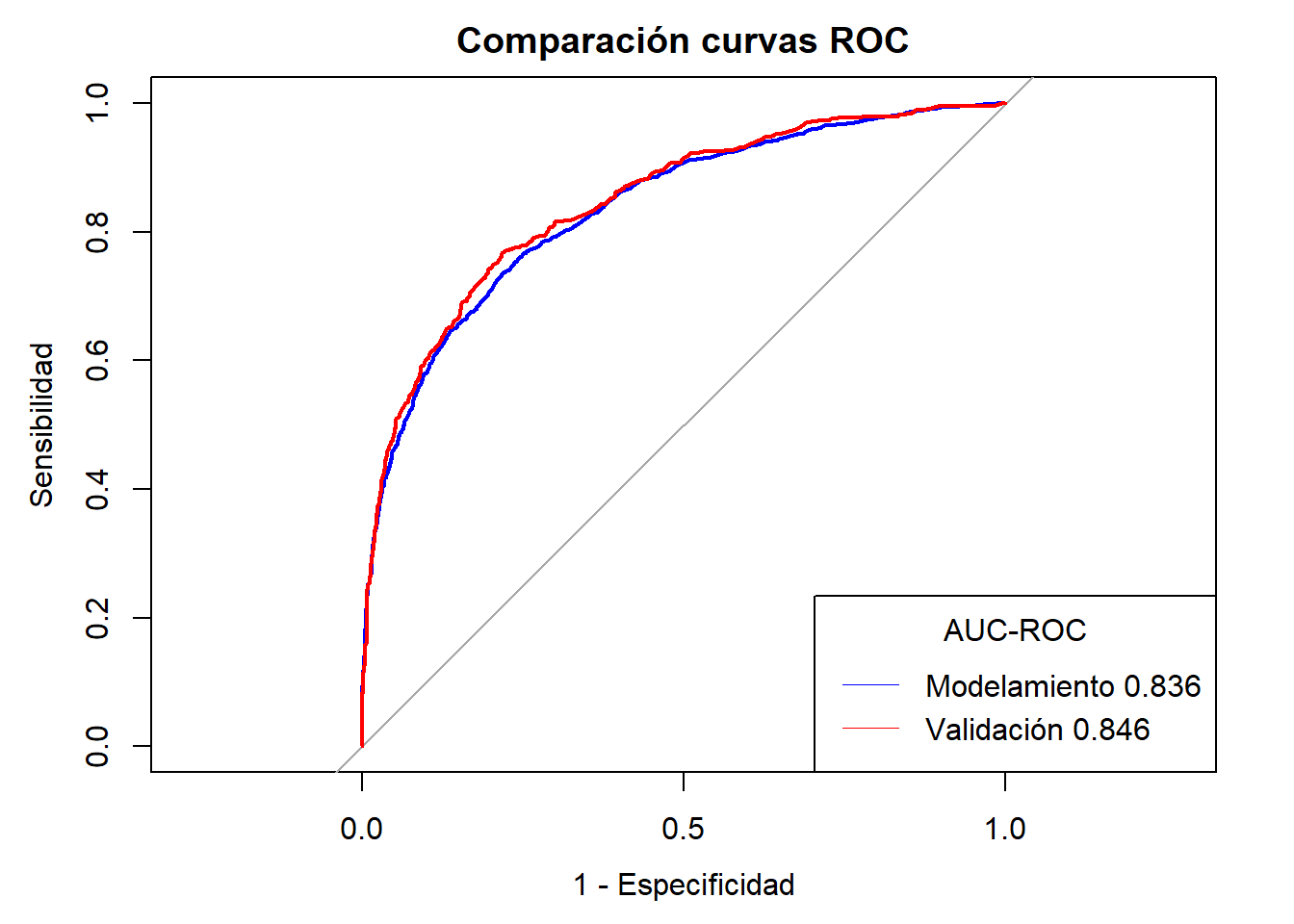
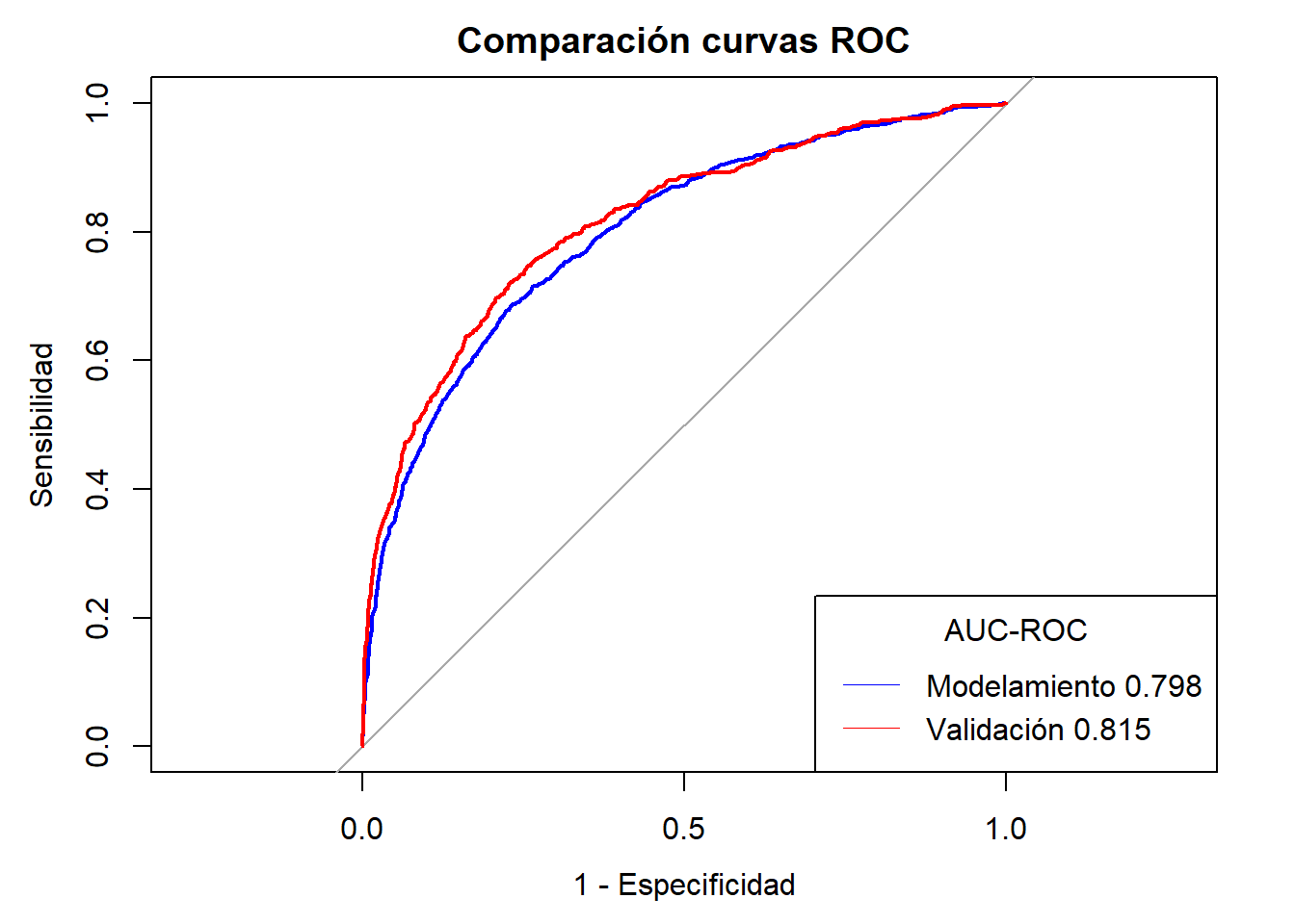
Con la librería scorecard se ha alcanzado un AUC-ROC de validación de 0.815

Ensamble

Creamos y damos formato necesario para utilizar h2o, nota en esta ocasión trabajaremos con las variables binneadas de forma personalizada

Código
# Ejecución del Ensamble

library(h2o)
h2o.init(ip = "localhost", nthreads = 2, max_mem_size = "5G")
 Connection successful!

R is connected to the H2O cluster: 
    H2O cluster uptime:         28 minutes 41 seconds 
    H2O cluster timezone:       America/Guayaquil 
    H2O data parsing timezone:  UTC 
    H2O cluster version:        3.44.0.3 
    H2O cluster version age:    8 months and 13 days 
    H2O cluster name:           H2O_started_from_R_joelb_nrn194 
    H2O cluster total nodes:    1 
    H2O cluster total memory:   4.91 GB 
    H2O cluster total cores:    8 
    H2O cluster allowed cores:  2 
    H2O cluster healthy:        TRUE 
    H2O Connection ip:          localhost 
    H2O Connection port:        54321 
    H2O Connection proxy:       NA 
    H2O Internal Security:      FALSE 
    R Version:                  R version 4.3.3 (2024-02-29 ucrt) 
Código
# Establecemos los datos en el formato adecuado
vars <- c("Exited", "prbm_NumOfProducts", "prbm_Age", "prbm_IsActiveMember", "prbm_Geography", "prbm_Gender", "prbm_EstimatedSalary")

mod_em <- as.h2o(x = setDT(mod)[, vars, with = FALSE])

  |                                                                            
  |                                                                      |   0%
  |                                                                            
  |======================================================================| 100%
Código
# Identificamos predictores y respuesta
y_em <- "Exited"; x_em <- setdiff(names(mod_em), y_em)

# Para la clasificación binaria, la respuesta debe ser un factor 
mod_em[,y_em] <- as.factor(mod_em[,y_em])

# Numero de CV folds 
nfolds <- 5

# Generaremos el ensamble con 3 modelos (RF + GLM + GBM)

Random Forest

Código
# Train & Cross- validate a RF
my_rf <- h2o.randomForest(x = x_em,
                          y = y_em,
                          model_id = "RF",
                          training_frame = mod_em,
                          ntrees = 300,
                          min_rows = 50,
                          mtries = 5,
                          nfolds = nfolds,
                          fold_assignment = "Stratified",
                          keep_cross_validation_predictions = TRUE,
                          seed = 95)

  |                                                                            
  |                                                                      |   0%
  |                                                                            
  |====                                                                  |   5%
  |                                                                            
  |=========                                                             |  12%
  |                                                                            
  |=======================                                               |  33%
  |                                                                            
  |============================                                          |  40%
  |                                                                            
  |==================================                                    |  49%
  |                                                                            
  |================================================                      |  68%
  |                                                                            
  |===================================================                   |  73%
  |                                                                            
  |==========================================================            |  83%
  |                                                                            
  |===============================================================       |  91%
  |                                                                            
  |======================================================================| 100%
Código
h2o.confusionMatrix(my_rf)
Confusion Matrix (vertical: actual; across: predicted)  for max f1 @ threshold = 0.239020037913721:
          0    1    Error        Rate
0      4556  989 0.178359   =989/5545
1       425 1028 0.292498   =425/1453
Totals 4981 2017 0.202058  =1414/6998

Gradient Boosting Machine

Código
# Train & Cross-validate a GBM
my_gbm <- h2o.gbm(x = x_em,
                  y = y_em,
                  model_id = "GBM",
                  training_frame = mod_em,
                  distribution = "bernoulli",
                  ntrees = 300,
                  max_depth = 5,
                  min_rows = 50,
                  learn_rate = 0.02,
                  nfolds = nfolds,
                  fold_assignment = "Stratified",
                  keep_cross_validation_predictions = TRUE,
                  seed = 95)

  |                                                                            
  |                                                                      |   0%
  |                                                                            
  |======                                                                |   8%
  |                                                                            
  |==============                                                        |  20%
  |                                                                            
  |============================                                          |  40%
  |                                                                            
  |====================================                                  |  52%
  |                                                                            
  |==================================================                    |  71%
  |                                                                            
  |========================================================              |  80%
  |                                                                            
  |=================================================================     |  93%
  |                                                                            
  |======================================================================| 100%
Código
h2o.confusionMatrix(my_gbm)
Confusion Matrix (vertical: actual; across: predicted)  for max f1 @ threshold = 0.324439576278591:
          0    1    Error        Rate
0      5050  495 0.089270   =495/5545
1       587  866 0.403992   =587/1453
Totals 5637 1361 0.154616  =1082/6998

Regresión Logística

Código
# Train & Cross-validate a GLM
my_glm <- h2o.glm(x = x_em,
                  y = y_em,
                  model_id = "GLM",
                  training_frame = mod_em,
                  alpha = 0.1, # penaliza inclusión excesiva de variables
                  remove_collinear_columns = TRUE,
                  nfolds = nfolds,
                  fold_assignment = "Stratified",
                  keep_cross_validation_predictions = TRUE,
                  seed = 95)

  |                                                                            
  |                                                                      |   0%
  |                                                                            
  |======================================================================| 100%
Código
h2o.confusionMatrix(my_glm)
Confusion Matrix (vertical: actual; across: predicted)  for max f1 @ threshold = 0.297621966238341:
          0    1    Error        Rate
0      4920  625 0.112714   =625/5545
1       569  884 0.391604   =569/1453
Totals 5489 1509 0.170620  =1194/6998

Ensamble RF + GBM

Código
# Train ensamble

e1m <- h2o.stackedEnsemble(x = x_em,
                           y = y_em,
                           training_frame = mod_em,
                           model_id = "Ensamble_1m",
                           metalearner_algorithm = "deeplearning",
                           base_models = list(my_rf, my_gbm))

  |                                                                            
  |                                                                      |   0%
  |                                                                            
  |======================================================================| 100%

Ensamble RF + RL

Código
e2m <- h2o.stackedEnsemble(x = x_em,
                           y = y_em,
                           training_frame = mod_em,
                           model_id = "Ensamble_2m",
                           metalearner_algorithm = "deeplearning",
                           base_models = list(my_rf, my_glm))

  |                                                                            
  |                                                                      |   0%
  |                                                                            
  |======================================================================| 100%

Ensamble RF + RL + GBM

Código
e3m <- h2o.stackedEnsemble(x = x_em,
                           y = y_em,
                           training_frame = mod_em,
                           model_id = "Ensamble3m",
                           metalearner_algorithm = "deeplearning",
                           base_models = list(my_rf, my_gbm, my_glm))

  |                                                                            
  |                                                                      |   0%
  |                                                                            
  |======================================================================| 100%

Predicciones

Código
# Realizamos los predicciones sobre la muestra de modelamiento / validación
mod_em <- as.h2o(x = setDT(mod)[, vars, with = FALSE])

  |                                                                            
  |                                                                      |   0%
  |                                                                            
  |======================================================================| 100%
Código
val_em <- as.h2o(x = setDT(val)[, vars, with = FALSE])

  |                                                                            
  |                                                                      |   0%
  |                                                                            
  |======================================================================| 100%
Código
mod_em[,y_em] <- as.factor(mod_em[, y_em])
val_em[,y_em] <- as.factor(val_em[, y_em])

res_f <- function(valida, resul){
  res <- data.frame(Exited = valida$Exited,
                    Exited_p = as.data.frame(resul)[,3],0)
  return(res)
} 

roc_graf <- function(res_mod, res_val, name=""){
objroc1 <- roc(res_mod$Exited, res_mod$Exited_p, auc=T, ci=T)
plot(objroc1, col="blue", xlab="1 - Especificidad", ylab="Sensibilidad", main=paste("Comparación curvas ROC",name), legacy.axes = TRUE)
objroc2 <- roc(res_val$Exited, res_val$Exited_p, auc=T, ci=T)
plot(objroc2, col="red", add=TRUE)
legend("bottomright", legend=c(paste("Modelamiento",round(objroc1$auc, 3)), paste("Validación", round(objroc2$auc, 3))), col=c("blue", "red"), lwd=0.5, title = "AUC-ROC")
}

Curva ROC RF

Código
# Random Forest
mod_rf <- setDT(res_f(mod, h2o.predict(my_rf, newdata = mod_em)))

  |                                                                            
  |                                                                      |   0%
  |                                                                            
  |======================================================================| 100%
Código
val_rf <- setDT(res_f(val, h2o.predict(my_rf, newdata = val_em)))

  |                                                                            
  |                                                                      |   0%
  |                                                                            
  |======================================================================| 100%
Código
roc_graf(mod_rf,val_rf, "RF")

Curva ROC RL

Código
# Regresión Logística
mod_glm <- setDT(res_f(mod, h2o.predict(my_glm, newdata = mod_em)))

  |                                                                            
  |                                                                      |   0%
  |                                                                            
  |======================================================================| 100%
Código
val_glm <- setDT(res_f(val, h2o.predict(my_glm, newdata = val_em)))

  |                                                                            
  |                                                                      |   0%
  |                                                                            
  |======================================================================| 100%
Código
roc_graf(mod_glm,val_glm, "Regresión Logística")

Curva ROC GBM

Código
# Gradient Boosting 
mod_gbm <- setDT(res_f(mod, h2o.predict(my_gbm, newdata = mod_em)))

  |                                                                            
  |                                                                      |   0%
  |                                                                            
  |======================================================================| 100%
Código
val_gbm <- setDT(res_f(val, h2o.predict(my_gbm, newdata = val_em)))

  |                                                                            
  |                                                                      |   0%
  |                                                                            
  |======================================================================| 100%
Código
roc_graf(mod_gbm,val_gbm, "Gradient Boosting")

Curva ROC RF + GBM

Código
# Ensamble RF + GBM
mod_e1m <- setDT(res_f(mod, h2o.predict(e1m, newdata = mod_em)))

  |                                                                            
  |                                                                      |   0%
  |                                                                            
  |======================================================================| 100%
Código
val_e1m <- setDT(res_f(val, h2o.predict(e1m, newdata = val_em)))

  |                                                                            
  |                                                                      |   0%
  |                                                                            
  |======================================================================| 100%
Código
roc_graf(mod_e1m,val_e1m, "Ensamble RF + GBM")

Curva ROC RF + RL

Código
# Ensamble GLM +RF
mod_e2m <- setDT(res_f(mod, h2o.predict(e2m, newdata = mod_em)))

  |                                                                            
  |                                                                      |   0%
  |                                                                            
  |======================================================================| 100%
Código
val_e2m <- setDT(res_f(val, h2o.predict(e2m, newdata = val_em)))

  |                                                                            
  |                                                                      |   0%
  |                                                                            
  |======================================================================| 100%
Código
roc_graf(mod_e2m,val_e2m, "Ensamble RF + GLM(RL)")

Curva ROC RL + RF + GBM

Código
# Ensamble GLM + RF + GBM
mod_e3m <- setDT(res_f(mod, h2o.predict(e3m, newdata = mod_em)))

  |                                                                            
  |                                                                      |   0%
  |                                                                            
  |======================================================================| 100%
Código
val_e3m <- setDT(res_f(val, h2o.predict(e3m, newdata = val_em)))

  |                                                                            
  |                                                                      |   0%
  |                                                                            
  |======================================================================| 100%
Código
roc_graf(mod_e3m,val_e3m, "Ensamble RF + GBM + GLM(RL)")

Conclusiones

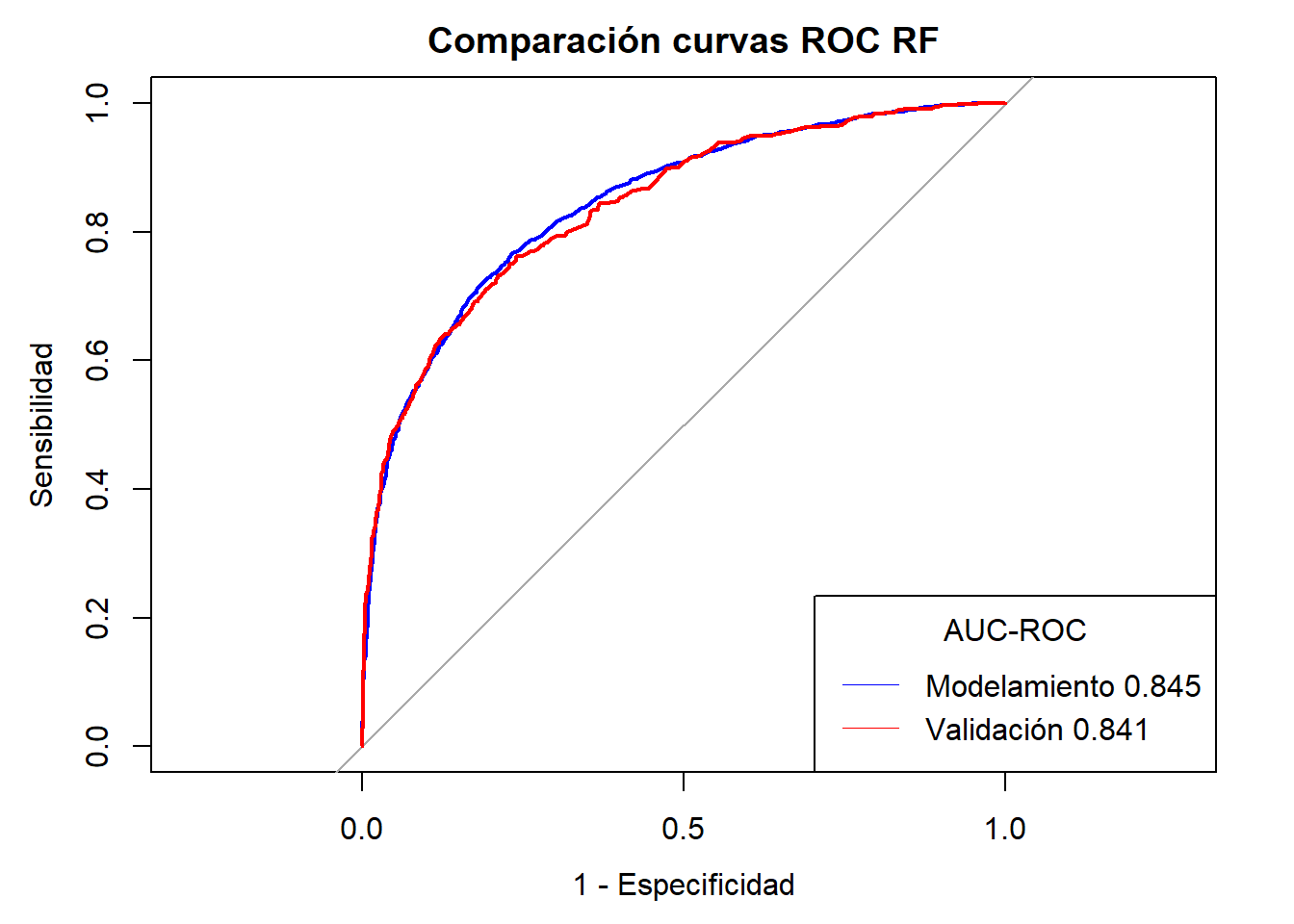
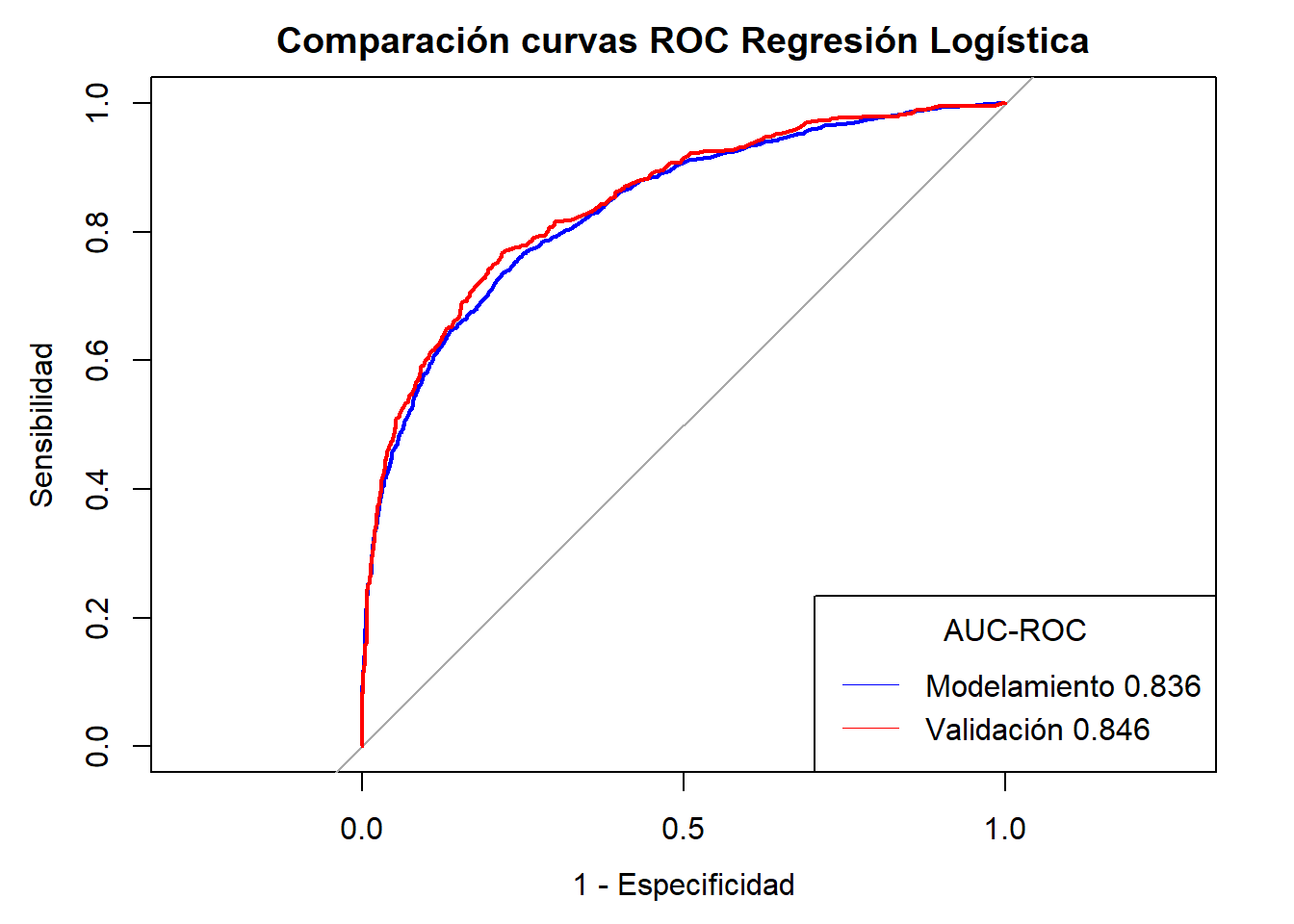
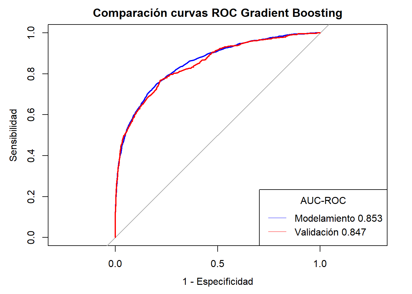
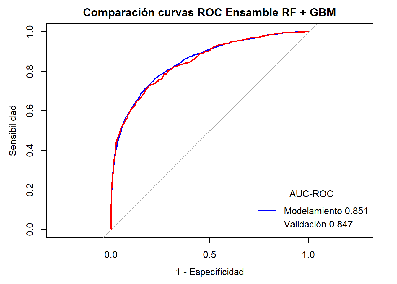
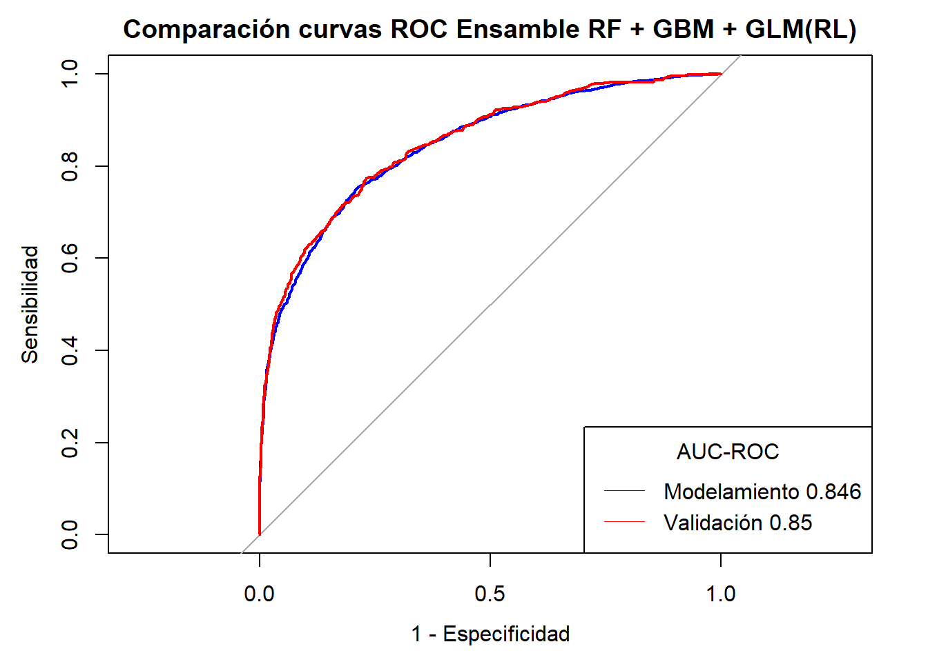
  • Notemos que en la mayoria de casos se ha alcanzado AUC-ROC \(\geq 0.80\) sin embargo el mejor modelo es el Ensamble de Random Forest + Gradient Boosting Machine + GLM( Regresión Logística) con una AUC-ROC validación de \(0.85\). Sin embargo el modelo también se ve sometido a requerimientos y recursos propios del negocio por lo que puede quedarse fuera y se opte por un modelo menos costoso en cuestión de tiempo y recursos.

Recomendaciones

  • En esta ocasión no hemos recurrido a una automatización completa del proceso de creación del modelo por lo que se podría explorar la creación de ensambles partiendo de las variables binneadas por optimal binning.